Predicting Player Market Valuation
April 15, 2026

Problem
Estimating player valuation is an important element in player recruitment and can help clubs to identify undervalued assets to optimize gains. This is the first step in exploring variables that can explain the player's market valuation
Key Insights
- • Age and player salary explains more than half of the variation in player market valuation
- • Using age, player salary, basic player's performance and in which league are they playing at achieves on average (adjusted) R-squared value of 0.77 on held-out test data using cross-validation method
- • Player position only had marginal impact to the model once other metrics are included. Prompts the notion that 'the highest valued players are attackers'
Tech Stack
Data Source
Transfermarkt; FootyStats
Motivation
We have seen how recruitment has played a big role in club’s succes, and notably, how clubs have spend big money in the transfer market. However, most clubs operate under strict budget. By establishing an objective and fair market value, recruitment teams can identify “undervalued” assets.
Player Market Valuation is an estimate of player’s transfer fee based on various factors such as age, performance, contract duration, and position.
In this project, I built a player market valuation prediction model using various publicly available player data (e.g., salary, age, perfomance, etc.).
The Data
I used publicly available dataset obtain from Transfermarkt and FootyStats website.
From Transfermarkt:
- Player market valuation (in million euros)
- On field metrics (goals, assist, number of appearance, minutes played)
- Player information (position, competition, club)
From FootyStats:
- Player annual salary (in million euros)
Data preparation:
- Obtain the 50 league highest earning players in each season from 2022 to 2025 from the top 5 European League (EPL, La Liga, Serie A, Bundesliga, Ligue 1)
- Match the salary information with the dataset obtain from Transfermarkt
- Player market valuation was done at various time during the year/season. For each player, I took the latest player’s valuation in a given season.
- Finally, for every player, I have their annual salary and market valuation for every season. Plus, their season performance metrics (e.g., total goals, total assist, total appearance) and the player profile information.
At the end, I had 839 data points across 392 unique players from 5 leagues to work with.
Modeling
I used a multiple linear regression to model the player market valuation.
First, I identify the predictors variable candiate from the dataset:
- annual salary
- age
- total goal (in a season)
- total assist (in a season)
- number of appearances (in a season)
- total minutes played (in a season)
- player’s position
- competition (the league that they are playing at)
- season (season identifier)
Variable tranformation
Upon exploring the dataset, I feel that it’s best to log transformed the salary, goal, assist, and market valuation data to manage some of the outliers.
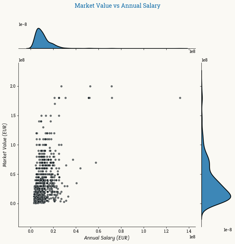
Example of variable relationships
Before transformation
After transformation 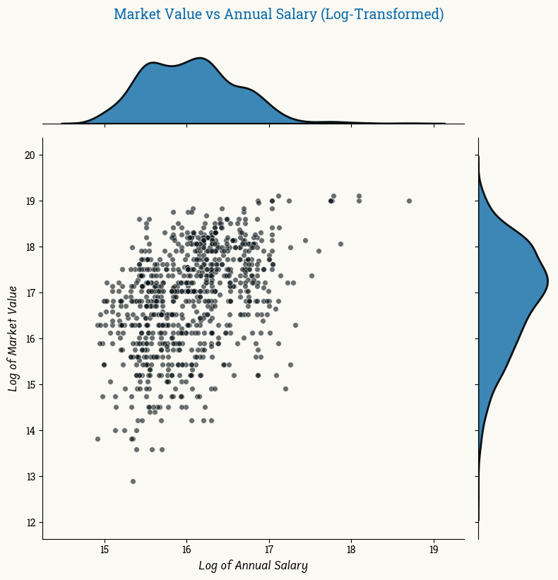
After transformation, the outliers data are closer to the rest of the sample.
Model evaluation
To evaluate the model, I use the (adjusted) R-squared is the main metric. I also include AIC and BIC as comparisons. To select the best model, I use the forward selection approach, in which we start with a simple model (1 predictor) and gradually add the most significant predictor until we don’t see improvement in the model performance anymore. Every model spefication is evaluated using cross validation with 5 folds. The model score is averaged throughout the 5 folds.
Show code: Forward Selection with cross validation
from sklearn.model_selection import cross_val_score
from sklearn.linear_model import LinearRegression
from sklearn.metrics import r2_score, mean_squared_error
import pandas as pd

def forward_selection(X, y, predictors, categorical_vars=None, scoring='r2', cv=5):
    """
    Forward selection with automatic handling of categorical variables.

    Parameters:
    -----------
    X : DataFrame
        Full dataset with all predictors
    y : Series
        Target variable
    predictors : list
        List of predictor names to consider
    categorical_vars : list
        List of categorical variable names
    scoring : str
        Scoring metric for cross-validation
    cv : int
        Number of cross-validation folds
    """


    if categorical_vars is None:
        categorical_vars = []

    selected_features = []
    remaining_features = predictors.copy()
    results = pd.DataFrame(columns=['Feature', 'CV R²', 'Adj R²', 'AIC', 'BIC'])

    while remaining_features:
        best_score = -np.inf
        best_feature = None

        for feature in remaining_features:
            # Create temporary feature list
            current_features = selected_features + [feature]

            # Prepare data with dummy variables
            X_temp = X[current_features].copy()

            # Create dummy variables for categorical features
            cat_features_in_current = [f for f in current_features if f in categorical_vars]
            if cat_features_in_current:
                X_temp = pd.get_dummies(X_temp, columns=cat_features_in_current, drop_first=True)

            # Handle missing values
            X_temp = X_temp.fillna(X_temp.mean())

            # Perform cross-validation
            model = LinearRegression()
            scores = cross_val_score(model, X_temp, y, cv=cv, scoring=scoring)
            score = scores.mean()

            if score > best_score:
                best_score = score
                best_feature = feature

        if best_feature:
            selected_features.append(best_feature)
            remaining_features.remove(best_feature)

            # Fit final model with selected features for metrics
            X_final = X[selected_features].copy()
            cat_features_selected = [f for f in selected_features if f in categorical_vars]
            if cat_features_selected:
                X_final = pd.get_dummies(X_final, columns=cat_features_selected, drop_first=True)

            X_final = X_final.fillna(X_final.mean())

            model = LinearRegression()
            model.fit(X_final, y)
            y_pred = model.predict(X_final)

            # Calculate metrics
            n = len(y)
            k = X_final.shape[1] + 1  # number of parameters
            r2 = r2_score(y, y_pred)
            adj_r2 = 1 - (1 - r2) * (n - 1) / (n - k)
            aic, bic = calculate_aic_bic(y, y_pred, k)

            # Store results
            print(f"\nIteration {len(selected_features)}:")
            print(f"Added feature: {best_feature}")
            print(f"Selected features: {selected_features}")
            print(f"CV R²: {best_score:.4f}, Adj R²: {adj_r2:.4f}, AIC: {aic:.2f}, BIC: {bic:.2f}")

            iteration_results = pd.DataFrame({
                'Feature': [str(selected_features.copy())],
                'CV R²': [best_score],
                'Adj R²': [adj_r2],
                'AIC': [aic],
                'BIC': [bic]
            })
            results = pd.concat([results, iteration_results], ignore_index=True)
        else:
            break

    return results
Results
Results of the models evaluation:
| Model | Feature | R2 | Adj. R2 | AIC | BIC |
|---|---|---|---|---|---|
| 0 | [‘Age’] | 0.3696 | 0.4196 | 2103.3735 | 2112.8379 |
| 1 | [‘Age’, ‘salary_log’] | 0.5783 | 0.6121 | 1766.3093 | 1780.5059 |
| 2 | [‘Age’, ‘salary_log’, ‘total_minutes’] | 0.694 | 0.7282 | 1468.7493 | 1487.6781 |
| 3 | [‘Age’, ‘salary_log’, ‘total_minutes’, ‘total_goals_log’] | 0.7195 | 0.7515 | 1394.5434 | 1418.2045 |
| 4 | [‘Age’, ‘salary_log’, ‘total_minutes’, ‘total_goals_log’, ‘competition_id’] | 0.736 | 0.7732 | 1322.0186 | 1364.6085 |
| 5 | [‘Age’, ‘salary_log’, ‘total_minutes’, ‘total_goals_log’, ‘competition_id’, ‘total_assists_log’] | 0.7364 | 0.7739 | 1320.5543 | 1367.8764 |
| 6 | [‘Age’, ‘salary_log’, ‘total_minutes’, ‘total_goals_log’, ‘competition_id’, ‘total_assists_log’, ‘total_appearances’] | 0.7357 | 0.7762 | 1312.9257 | 1364.98 |
| 7 | [‘Age’, ‘salary_log’, ‘total_minutes’, ‘total_goals_log’, ‘competition_id’, ‘total_assists_log’, ‘total_appearances’, ‘position’] | 0.7347 | 0.7773 | 1311.7642 | 1378.0151 |
| 8 | [‘Age’, ‘salary_log’, ‘total_minutes’, ‘total_goals_log’, ‘competition_id’, ‘total_assists_log’, ‘total_appearances’, ‘position’, ‘season’] | 0.729 | 0.8068 | 1196.3338 | 1281.5136 |
What the model tells us
- The most informative predictors were age and salary. Together they explain 61% of variance.
- Playing time actually adds more significant value than goals and assist. This may be because this metric is not relevant for all position.
The results show that the model plateaued around 6-7 features (Adj. R² ~0.77). We see that from model 6 onwards, the performance starts to decline or don’t improve much. Arguably, the best model is the model 7 with features: ‘Age’, ‘salary_log’, ‘total_minutes’, ‘total_goals’, ‘competition_id’, ‘total_assists’, ‘position’, and ‘appearances’. However, the improvement is not much more significant than model 5. If simplicity and explanability is a priority, using model 5 may be sufficient.
Next Steps and Future Research
- Include a bigger sample of players. Currently, the sample is limited to the players with the highest earnings in the league.
- Incorporate other potentially relevant variables:
- remaining length of the players contract
- other relevant on field performance and team results
- players’ commercial appeal
- Compare model predictions against actual transfer price